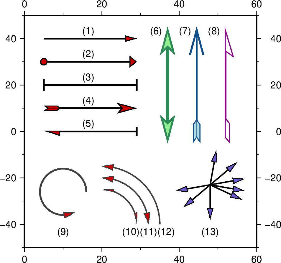
Vectors

The pygmt.Figure.plot method can plot three classes of vectors: Cartesian, circular and geographic. While their use is slightly different, they all share common modifiers that affect how they are displayed. We must specify the vector type and the modifiers by passing the corresponding shortcuts listed below to the style argument. Additionally, we must define the vector directions (angle and length, azimuth and length, or x and y components) via the direction argument.

The following vectors are available:

• v: cartesian

• m: circular (math angle arc)

• =: geographic

Upper-case versions V and M are similar to v and m but expect geographic azimuths and distances.

import numpy as np
import pygmt

fig = pygmt.Figure()
fig.basemap(region=[0, 60, -50, 50], projection="X10c/10c", frame=True)

Plot simple horizontal vectors (1)-(5)

x = 5
y = 40
idx = 1

for vecstyle in [
    "v0.5c+e",  # (1) simple vector (angle of 0 degrees and length of 4) with arrow head at the end
    "v0.3c+bc+ea+a80",  # (2) vector with arrow head at the end and a circle at the beginning
    "v0.3c+bt+et+a80",  # (3) vector with terminal lines at beginning and end
    "v0.85c+bi+ea+h0.5",  # (4) vector with tail at the beginning and an arrow with modified vector head at the end
    "v0.7c+bar+et",  # (5) vector with half-sided arrow head at the beginning and terminal line at the end
]:
    fig.plot(x=x, y=y, style=vecstyle, direction=([0], [4]), pen="2p", color="red3")
    fig.text(x=16.5, y=y + 3.5, text="(" + str(idx) + ")")
    y -= 10  # move the next vector down
    idx += 1

Plot simple vertical vectors using different pens and colors (6)-(8)

x = 37
y = -5

vectorsv = [
    ["v1.2c+e+b+h0.5", "lightgreen", "4p,seagreen"],  # (6)
    ["v1.2c+bi+eA+h0.2", "lightblue", "2p,dodgerblue4"],  # (7)
    ["v1.3c+bi+ea+h0.4+r", "white", "2p,darkmagenta"],  # (8)
]

for vector in vectorsv:
    fig.plot(
        x=x, y=y, direction=([90], [5]), style=vector[0], color=vector[1], pen=vector[2]
    )

    fig.text(x=x - 3, y=43.5, text="(" + str(idx) + ")")

    x += 7.5
    idx += 1

Plot circular vectors (9)-(12)

# (9) plot a math angle arc with its center at 10/-26,
#     a radius of 1 and a start angle of 0 and end angle of 300 degrees
data = np.array([[10, -26, 1, 0, 300]])
fig.plot(data=data, style="m0.5c+ea", color="red3", pen="2p,gray25")

fig.text(x=10, y=-43, text="(" + str(idx) + ")")
idx += 1

# (10-12) plot math angle arcs starting at 0 degrees and ending at 90 degrees
#         with different radii and start/end vector modifiers
x = 20
y = -40
startdir = 0
stopdir = 90
radius = 1.5
pen = "1.5p,gray25"
xtext = 24.5

for arcstyle in [
    "m0.5c+ea+ba+r",  # (9) right-sided half-arrow heads at beginning and end
    "m0.5c+ea+ba",  # (10) arrow head at beginning and end
    "m0.5c+ea",  # (11) arrow head at the vector end
]:

    data = np.array([[x, y, radius, startdir, stopdir]])
    fig.plot(data=data, style=arcstyle, color="red3", pen=pen)

    fig.text(x=xtext + 3, y=-43, text="(" + str(idx) + ")")

    radius += 0.5
    xtext += 4.55
    idx += 1

Plot set of vectors with arrow ends starting from one center point (13)

x = np.repeat(48, 8)
y = np.repeat(-23, 8)
lengths = np.repeat(1.5, 8)

fig.plot(
    x=x,
    y=y,
    direction=([80, 50, 10, 100, 260, 115, 180, 230], lengths),
    style="V0.5c+e",
    color="slateblue",
    pen="1.5p",
)

fig.text(x=48, y=-43, text="(" + str(idx) + ")")

fig.show()

Out:

<IPython.core.display.Image object>